Molecular water detected on the sunlit Moon by SOFIA
Abstract
Widespread hydration was detected on the lunar surface through observations of a characteristic absorption feature at 3 µm by three independent spacecraft1,2,3. Whether the hydration is molecular water (H2O) or other hydroxyl (OH) compounds is unknown and there are no established methods to distinguish the two using the 3 µm band4. However, a fundamental vibration of molecular water produces a spectral signature at 6 µm that is not shared by other hydroxyl compounds5. Here, we present observations of the Moon at 6 µm using the NASA/DLR Stratospheric Observatory for Infrared Astronomy (SOFIA). Observations reveal a 6 µm emission feature at high lunar latitudes due to the presence of molecular water on the lunar surface. On the basis of the strength of the 6 µm band, we estimate abundances of about 100 to 400 µg g−1 H2O. We find that the distribution of water over the small latitude range is a result of local geology and is probably not a global phenomenon. Lastly, we suggest that a majority of the water we detect must be stored within glasses or in voids between grains sheltered from the harsh lunar environment, allowing the water to remain on the lunar surface.
Main
Using SOFIA and the Faint Object infraRed CAmera for the SOFIA Telescope (FORCAST) instrument, we conducted observations of the lunar surface at 6 µm on 31 August 2018 in a search for molecular water. FORCAST is well suited to look for 6 µm lunar water due to its wavelength coverage from 5 to 8 µm, spectral resolution of R = 200 and high signal-to-noise ratios. The FORCAST entrance slit that defines the portion of the Moon observed is 2.4 × 191 arcsec sampled with 248 pixels. At the lunar centre of disk the slit has a spatial extent of 4.8 × 1.5 km2 (the spatial resolution near the limb is lower due to foreshortening). During the observations, the Moon was at a phase angle of 57.5°. We observed a region at high southern latitudes near Clavius crater and a low-latitude portion of Mare Serenitatis (Extended Data Fig. 1). Details regarding observations, site selection and data reduction can be found in the Methods. Data from SOFIA reveal a strong 6 µm emission band at Clavius crater and the surrounding terrain (Fig. 1) relative to the control location near the lunar equator, which shows low hydration in some analyses (see Methods). All spectra from the Clavius region exhibit this 6 µm emission feature. The majority of these emission peaks (98%) exceed 2σ significance relative to the background noise, and about 20% exceed 4σ significance (Extended Data Fig. 2).
Fig. 1: Lunar 6 µm emission bands.

Spectra of the Clavius region show a strong 6 µm emission band, indicating the presence of H2O at the locations noted in the top right corners (Clavius frame numbers are noted in the top left corners). Abundances derived from these spectra range from 100 to 400 µg g−1 H2O. Abundance and location information can be found in Supplementary Tables 1 and 2. The error bars indicate 1σ uncertainty.
To determine whether the spectral properties of the lunar 6 µm band are consistent with spectra of particulate water-bearing materials, we examined other planetary materials that show a 6 µm H2O band. We compared our measurements to literature values of the centre position of the H–O–H bend in crystalline hydrates6, the 6 µm band centres and widths of spectra of a water-bearing mid-ocean-ridge basalt (MORB) glass7 and to meteorites with water adsorbed from the terrestrial environment8. For each lunar spectrum, we fit the emission peak with a Gaussian function and report the band centres (Fig. 2) and widths in Table 1.
Fig. 2: 6 µm band centre frequency distribution.
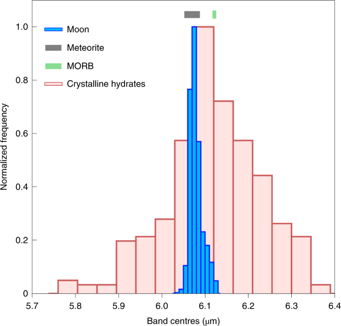
6 µm band centres of the lunar, meteorite and MORB spectra and the observed centre position of H–O–H of crystalline hydrates from Falk6. The meteorite and MORB data are shown as ranges and have sample sizes of 4 and 5, respectively.
Table 1 6 µm band properties
The observed band centres for the Moon, meteorites and MORB glass all fall near the mode of the reported band centre range of the H–O–H bend in crystalline hydrates6 (Fig. 2). The Moon and meteorite band centres vary more than those of the MORB glass and are slightly offset; this is not unexpected because the glass spectra are from a single sample that has been heated step-wise to drive off water incrementally9. Variation in hydrogen bonding of water in the host materials can account for the differences among the samples. The peak widths are also consistent among the Moon, meteorites and MORB glass, with strong overlap among the distributions (Table 1). On the basis of these comparisons, we attribute the observed 6 µm feature on the Moon to molecular water. We are unaware of any other material reasonable for the Moon that exhibits a single spectral feature at 6 µm other than H2O.
We then used the lunar emission peak intensities to estimate the abundance of water at our observed locations (see Methods). In a laboratory analysis of geologic thin sections, the abundance of H2O is quantified by measuring the 6 µm absorbance peak height, controlling for the thickness of the sample and converting these to abundances using the Beer–Lambert law and measured molar extinction values for water4. In remote sensing of planetary regolith, surfaces are in particulate form and no work has been done on deriving the absolute abundance of H2O from spectra of particulates near 6 µm. However, in previous work, Li and Milliken7 derived a calibration between the abundance of water and the intensity of the 3 µm band in reflectance using spectra of a particulate water-bearing MORB glass with a known absolute water content. Using this same sample set and approach, we used the 6 µm band intensities in the glass to derive an empirical relationship between band depth in reflectance and absolute abundance of H2O (Extended Data Fig. 3). The empirical relationship is:
Mwater=9,394D2band+9,594Dband,Mwater=9,394Dband2+9,594Dband,
(1)
where Mwater is the abundance of H2O (in µg g−1) and Dband is the depth of the 6 µm band.
Derived abundances in the Clavius region range from about 100 to 400 µg g−1 H2O with a mean of about 200 µg g−1 H2O. These estimates are lower limits because the lunar mare equatorial site was used as the reference (hereafter referred to as the mare reference) and any water present there would have been removed from the Clavius data during the calibration process (see Methods). The error in abundance is about 80 µg g−1 H2O based on the statistical noise in the data, and including errors from the uncertainty in lunar emissivity used in the calibration (see Methods).
An outstanding problem since the discovery of the 3 µm absorption is how much of that feature is due to molecular water and how much is due to hydroxyl. At present, the 3 µm band cannot be used to distinguish between molecular water and hydroxyl. To begin to understand the relative abundances of water and hydroxyl, we directly compare our molecular water abundances with total water abundances (OH + H2O) derived from the Moon Mineralogy Mapper (M3) for the regions sampled by the SOFIA FORCAST slit in Fig. 3. We note that there has been disagreement regarding the distribution of total water based on removal of thermal emission from M3 data. For example, three studies7,10,11 report decreases in band depth and total water content towards the equator, whereas one study12 used a different data reduction approach and reported no drop in band intensity towards the equator. All four groups, however, agree on high band depths at high latitudes where emitted radiance is lowest, lending confidence to the total water abundances in the Clavius region reported by Li and Milliken7. This agreement provides support for our derived abundances using 6 µm observations due to the similar abundances in total water from M3 and molecular water from SOFIA.
Fig. 3: Latitude variations.
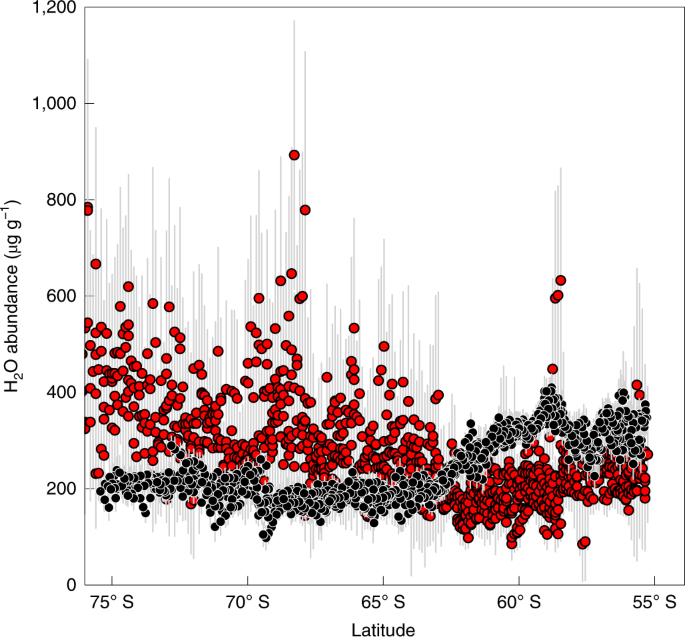
Abundances versus latitude measured by SOFIA at 6 µm (black) and M3 at 3 µm (red; M3 units are H2O equivalent). The grey lines are 1σ uncertainties in the M3 data. Abundances measured by SOFIA fall within 1σ of M3 total water abundances.
The abundances estimated from SOFIA all fall within 1σ of the M3 data, however, the trends of total water from M3 and molecular water from SOFIA with latitude are different. In the lower-latitude SOFIA data below about 65°, both our data and M3 lie on the ejecta blanket of Tycho crater. Both total water and molecular water show relatively constant values, with SOFIA abundance estimates around 300 µg g−1 H2O and M3 total water estimates around 200 µg g−1 H2O. Off Tycho’s ejecta towards the south, M3 total water values steadily increase from about 200 to about 400 µg g−1 H2O, whereas SOFIA molecular water abundances are constant around 200 µg g−1 H2O. The observed trend with latitude in this specific region may be due to the local geology rather than a general global phenomenon (see Methods). The cause of the differences in the spatial distribution of abundances is not clear. The two wavelength regions are not probing precisely the same portions of regolith grains and depths in the regolith; these differences may therefore reflect variations in the location of hydroxyl and molecular water in the regolith grains. For example, the depths of the 3 and 6 µm bands show good correlation in laboratory samples, but they are not exactly correlated. More data are required to address this issue. Other possible reasons for the differences between SOFIA and M3 datasets are discussed in the Methods (see the Extended discussion on estimated abundances in the Clavius region section).
There are several mechanisms for the origin of water in lunar soil that are relevant to our data. Water present in the lunar exosphere can be chemisorbed on grain surfaces13. Water can be introduced by volatile-rich micrometeorites, and a portion of this water can be retained in the glasses resulting from these impacts14 or introduced into the exosphere, available for chemisorption15. Water can be formed in situ on grain surfaces from pre-existing hydroxyl that undergoes recombinative desorption at high lunar noontime temperatures, particularly at the equator, also releasing this water into the exosphere for later loss or trapping16. Water can also be formed in situ from pre-existing hydroxyl during micrometeorite impact, when high temperatures promote the reaction, as has been recently demonstrated in the laboratory17. In experiments, the water was detected as vapour, but presumably a portion of that water can also be sequestered into impact glasses.
Chemisorbed water is unlikely to be a substantial portion of our signal. Poston et al.18 modelled the amount of molecular water that would be present on grain surfaces after several lunations and showed that only 3 µg g−1 of H2O can reside on the surface of grains at the derived brightness temperature, lunar time of day and latitudes of our observations (see Methods). Similarly, Hendrix et al.19 estimate that about 1% of a monolayer of molecular water is present if the diurnal variation in the UV water-ice band ratio is due to water, which corresponds to only a few µg g−1 of water. This almost certainly means that the water detected by SOFIA resides within the interior of lunar grains or is trapped between grains shielded from the harsh lunar environment, allowing it to survive a lunation. However, observations with SOFIA cannot distinguish between water within impact glasses and water trapped between grains and within void spaces. (We note that the lunar band centres are more similar to those of adsorbed water in the meteorite spectra than to the internal water in a single water-bearing glass spectrum. There are, however, few data available to confidently conclude that the band centre is an indicator of the location of water on or within grains. We instead rely on the physical chemical models that strongly exclude chemisorbed water). Lastly, the minerals that make up a large fraction of lunar soil are nominally anhydrous and should have extremely low water contents20. For these reasons, we conclude that the water we observe is trapped within impact glasses.
Assuming that the water resides within glasses, we estimate the abundance of water within the glass itself. Most lunar soil comprises a combination of about 30 wt% glass derived from micrometeorite impact21 and the remainder being rock and mineral fragments. If our observed water is confined to impact glass, then taking the abundance of water measured in our spectra and dividing it by 30%, the abundance of water within impact glasses ranges from about 300 to 1,300 µg g−1 H2O with an average of 700 µg g−1 H2O. Daly and Schulz14 performed impact experiments with water-bearing projectiles and found molecular water in their experimentally produced impact glass at abundances of 215 to 7,698 µg g−1 H2O using Fourier transform infrared measurements at 6 µm; our estimated water abundances within impact glass lie within this range. Our estimated mean abundance of water in glass is about four times higher than the total water in micrometeorite impact glasses measured by Liu et al.22, who reported 70–170 µg g−1 H2O equivalent in Apollo lunar soil samples that are all from low-latitude sites.
The similar abundances of molecular water and total water (Fig. 3) indicate that little hydroxyl is present at the lower latitudes that we observed (latitudes from ~65° to 55°). Impactor water entrained in impact glass explains this observation, but our data do not exclude in situ conversion of hydroxyl to water. However, if this occurs, the conversion from hydroxyl to water is highly efficient. Hydroxyl is expected at all latitudes due to solar wind exposure23,24,25,26, so our results suggest that the micrometeorite flux, at least at the latitudes observed, is sufficient to process much of the hydroxyl that is present to water. Models of the rate of hydroxyl formation are highly dependent on the distribution of activation energies available and hydroxyl formation processes27, so our observations provide a useful constraint on models for the chemistry of hydrogen in lunar soils, and by extension other planetary surfaces.
Our results are more consistent with the existence of a mechanism that produces water by impact from pre-existing lunar material, perhaps the mechanism of Zhu et al.17, than impact-delivered water. Analysis of data taken near the equator by the Lunar Atmosphere and Dust Environment Explorer (LADEE) suggests that smaller impacts that probe the upper few centimetres of the regolith do not result in water released to the exosphere and that the uppermost few centimetres of soils are desiccated15. LADEE results also show that the impacts that do result in exospheric water exsolve more water than the impactor can contain. The LADEE result is consistent with the low equatorial total water estimates7 and the weak equatorial 3 µm bands10,11. The low water abundances that we find at the mare reference near the equator are consistent with the LADEE result of a desiccated layer. Contrary to LADEE measurements confined to the equator, our results show that soils at high latitudes (or at least at our high-latitude locations) are not desiccated, supporting several models16,27,28 that suggest a depletion of hydroxyl at the equator and an increase in hydroxyl at higher latitudes. Our result suggests that this high-latitude hydroxyl is efficiently processed to molecular water and sequestered in glass.
Our data are a snapshot at one location and time on the Moon and so cannot address diurnal timescales or the timescales of the evolution of molecular water. Future 6 µm observations similar to UV observations19 could constrain diurnal variations in molecular water across the lunar surface, and more extensive latitudinal and spatial coverage could also separate local geologic variations from general latitudinal trends.
Methods
Lunar observations with SOFIA
SOFIA is a 2.5 m telescope flown on a Boeing 747-SP aircraft used for infrared and submillimetre astronomy29. The FORCAST instrument combines a spectrograph and a mid-infrared camera using a 256 × 256 Si Blocked-Impurity-Band infrared focal plane array30. For lunar observations, we used the FORCAST G063 filter with the long-slit (2.4 × 191″) low-resolution mode to provide a spectral coverage of 5 to 8 µm. With a slit width of 2.4″ and 0.768″ pixel height, the spatial resolution of a pixel at the lunar centre of disk is 4.8 × 1.5 km2. Near the limb, foreshortening causes the spatial pixel size along the slit to increase with the cosine of the emergence angle, assuming a smooth spherical Moon.
Two sunlit locations on the Moon were observed: a region at high latitude to search for water where total water has been reported to be high7 and, as a control, an equatorial region that was expected to have little H2O. Both locations were observed on the same SOFIA flight within a 10 min period. At the high-latitude site, an integration time of 4.16 s per frame was used and at the equatorial site 3.8 s per frame. A total of 12 frames were acquired, 6 for each location. The zenith angle of the observations was ranged from 33.06° to 33.54° between the two observed locations and the aircraft travelled less than ~1.5° in terrestrial longitude and maintained an altitude between 13,105 m and 13,112 m during the observations. Supplementary Table 1 provides the parameters of each frame and the flight condition with which they were acquired.
At high southern latitudes, the slit was placed from the lunar limb through the region near the crater Clavius (Extended Data Fig. 1). This location was chosen because it shows high total water abundances in M3 data7 and thus molecular water was possible. M3 data at 3 µm measure total water but are reported as equivalent H2O; they do not necessarily indicate the presence of H2O due the current inability to distinguish between OH and H2O using data at 3 µm. For the Clavius observations, the slit begins on the Moon and extends to the limb of the Moon and off into sky (Extended Data Fig. 1). The lunar local hour varied from 14:19 at 28.6° W, 75° S to 15:39 at 8.59° W, 55.6° S.
At low latitudes, we use a location in Mare Serenitatis (Extended Data Fig. 1) to represent a location with possibly little to no H2O present. Li and Milliken7 report no hydration for a majority of this observed location, but high total water at a pyroclastic deposit at one end of our slit. This region is excluded from our reference owing to the possibility of the presence of molecular water. For the above reasons, we use the Mare Serenitatis location as a reference. The lunar local hour was ~ 17:00. Both the Clavius and mare reference locations are prominent on the lunar surface, which aided in locating each feature in guider images used to support FORCAST target acquisition.
SOFIA pipeline processing
We received fully calibrated flux data from SOFIA. The data are in the form of spectral images that are 248 × 248 pixels, where the x axis is wavelengths covering 5 to 8 µm and the y axis is the spatial position on the Moon along the spectrograph slit. Data were processed using the standard SOFIA corrections30. The processing steps are shown in Supplementary Fig. 1, and include the removal of bad pixels, droop effect correction (the readout electronics exhibit a response offset, causing a reduction in artefacts), nonlinearity correction (to linearize the response of the detector), stacking (background subtraction of sky observations) and jailbar removal (the removal of any residual signal in the raw data that creates stripes in the spectral frame). Because the Moon fills the entire FORCAST slit, the full spectral image was processed without spectral extraction. The processing, therefore, skips the extract and merge steps and continues to the flux calibration (Supplementary Fig. 1).
In the flux calibration step, each spectrum is corrected for instrumental response and atmospheric transmission. At its operational altitude near 43,000 ft, spectra collected by SOFIA are not completely free from telluric water vapour absorption lines, and water is typically present at abundances of ~2–10 µg g−1 (ref. 31). The SOFIA processing pipeline corrects for the atmospheric opacity and water vapour so that images taken at different atmospheric conditions, altitudes or zenith angles can be combined32. Each individual spectral image and its atmospheric conditions are corrected using the atmospheric transmission (ATRAN) model32,33 to produce a look-up table of models. The ATRAN models are computed for every 1,000 ft in altitude from 35,000 ft to 45,000 ft, for every 5° of zenith angle between 30° and 70°, and for a range of precipitable water vapour (PWV) values between 1 and 50 µm (ref. 32). The model spectra are smoothed to match the spectral resolution of FORCAST (R = 200) and then the best estimate of the telluric absorption spectrum is detected and is divided out of the observed spectrum, yielding a telluric-corrected and flux calibrated spectrum in units of jansky32. The SOFIA pipeline selected the same atmospheric model for all 12 frames of data collected with model parameters of 43,000 ft, 35° zenith angle and 4 µm PWV. Selection of the same model suggests that the atmosphere was stable over the course of our observations within the quantization of the look-up table.
Removal of instrument artefact
Spectral images we received from FORCAST show a low-frequency spectral oscillation (Supplementary Fig. 2) that has been observed in previous FORCAST data. The oscillation appears in all frames of data acquired at both the Clavius and mare reference regions. The observed oscillation is nearly identical for both regions and is an instrument artefact and is not due to spectral variation of the lunar surface. The 6 µm emission that we show in Fig. 1 is relatively weak and is on the same order of intensity as the spectral oscillation artefact. Therefore, the oscillation must be removed to properly analyse the data. To remove it, we use the six mare reference spectral images at low latitude (that is, negligible OH + H2O abundance) to isolate the oscillation. There is an artefact in the top right corner due to contamination on the FORCAST detector; the spectra in these rows are avoided during processing and interpretation.
To characterize the oscillation observed in the spectral images, we first remove a continuum from each spectrum (image row) in all six of the acquired mare reference spectral images (Supplementary Fig. 3a and b). Then we take the mean of the continuum-removed images to create an image of the oscillation (Supplementary Fig. 3c) and divide it out of the Clavius spectral images to provide clean spectral images (Supplementary Fig. 4b). The removal of the continuum sets the oscillation image to have a mean about 1 so that when the oscillation image is divided out of the Clavius spectral images, the flux values are preserved. Application of the oscillation correction to the Clavius data uses only the section of the slit that was on the mare in the mare reference data (because one end of the Clavius slit falls onto the sky) and did not include the pyroclastic-draped highland material at the edge of the slit in the mare reference (Supplementary Fig. 2). Supplementary Fig. 4 shows Clavius spectral images before and after the oscillation is removed. On visual inspection of the spectral image with the oscillation removed, we see that the oscillation has largely been mitigated. Some residual oscillation, however, does remain, as seen at the bottom of the Supplementary Fig. 4b. Supplementary Fig. 5 shows a spectrum from the mare reference showing no band at 6 µm. It is unknown whether there is H2O present at the mare reference location, therefore, if there is H2O present, the oscillation image will cancel out whatever water emission is present in the Clavius data. For this reason, we report lower-limit abundances of H2O at the Clavius region.
After removing an instrument artefact, we convert flux to radiance and remove a linear continuum around the band using wavelengths 5.7–5.8 µm and 6.3–6.4 µm (avoiding the wavelengths of the band itself) from each spectrum. Supplementary Fig. 6 shows a spectrum from the Clavius region at a longitude and latitude of 14.5° W and 55.5° S with the oscillation, with the oscillation removed and with the oscillation and linear continuum around the band removed and a Gaussian function over plotted (supplementary Fig. 6a,b and c, respectively). A 6 µm band can be seen after artefact removal, superimposed on the continuum (Supplementary Fig. 6b), and is clearly seen after the continuum is removed (Supplementary Fig. 6c).
Significance of the observed 6 µm bands
All spectral images of the Clavius region show a 6 µm emission band (Supplementary Fig. 7). In each spectral image, the 6 µm band is broad and qualitatively similar spatially (along the slit).
To assign a level of confidence to the observed 6 µm emission bands, we calculated the Z score for the band observed in each spectrum. The Z score is defined as:
Z=x−μσZ=x−μσ
(2)
where µ is the average continuum value of each spectrum between wavelengths 5.5 µm and 7.5 µm while avoiding the 6 µm band region between 5.8 µm and 6.3 µm, σ is the noise of each spectrum found from the standard deviation of the continuum range used for µ and x is the peak height found by taking the mean of 0.1 µm about the 6 µm band centre, which is found by fitting each spectrum with a Gaussian function to find the 6 µm band centre, width and depth. Extended Data Fig. 2 shows the Z score histogram distribution for all six Clavius spectral frames; 98% of the spectra show a confidence level above the 95% confidence level.
Effectiveness of atmospheric water removal
To provide confidence in the telluric correction performed by the SOFIA pipeline and ensure that the peak we are observing is not due to residual atmospheric water, we generated multiple ATRAN models (https://atran.arc.nasa.gov/cgi-bin/atran/atran.cgi), ranging from 0.01 µm PWV (essentially no atmospheric water) to the 5 µm PWV (4 µm PWV was selected by the SOFIA pipeline as the best fit). All models were generated for 43,000 ft, the closest altitude during our observations and the altitude the SOFIA pipeline chose as the best fit, and a zenith angle of 33° (Supplementary Table 1). To see the effect of small errors in the estimation of water abundance, we made transmission ratios with different PWV values to rule out the possibility of residual PWV creating an apparent 6 µm emission band. We use PWV transmission ratios of 4 to 3, 3.25, 3.5, 3.75 and 5 µm PWV and compared it to a spectrum from Clavius that shows a strong 6 µm band (Supplementary Fig. 8). Ratio spectra of models with varying water abundances are clearly different from the emission feature we detected. In the Clavius spectrum there is only one band around 6 µm, whereas in the ratio spectra for 3 to 3.75 µm PWV, there are always two clusters of peaks for PWV errors near 6 µm and 6.5 µm. If any atmospheric water spectral features remained in our lunar data they would have to exhibit both the 6 µm and 6.5 µm water vapour peaks. If more PWV was removed than was present, as in the scenario for 4 µm PWV to 5 µm PWV, then an apparent broad peak occurs at ~6.3 µm. In comparison with the Clavius spectrum, the ratio spectrum has a broader peak with a band centre at longer wavelengths. This comparison gives us confidence that we are not detecting terrestrial water and that the 6 µm band on the Moon is in fact due to lunar water. To isolate the PWV and remove all other atmospheric lines, we took the ratio of the 4 µm PWV and 0.01 µm PWV models (Supplementary Fig. 9). Here we see a line at 7.7 µm is removed in the ratio (Supplementary Fig. 9b), this line is due to terrestrial methane. We can see the remaining spectral features are due to PWV, which has two distinct peak regions around 6 µm and 6.5 µm.
Estimated water abundances
Given that we have established that the 6 µm emission bands are statistically significant, and that we assigned that peak to water in solids in the main text by comparison to spectral parameters of other water-bearing materials and confirmed the band is not residual atmospheric water, the next challenge is to estimate the abundances of water from the emission peak intensity. To do this, we rely on a set of diffuse reflectance spectra of a particulate glass sample with well-known water concentrations to derive a calibration of absorption intensity to water abundance. We convert our data observed in emission to reflectance via Kirchhoff’s Law using assumptions regarding the emissivity of our Clavius site to apply the calibration curve.
Decades of studies show that the absorption strength of the 6 µm band correlates with the absolute H2O content34,35,36. Since the 1960s the 6 µm band has been used to measure the H2O content of samples in thin section in chemical and geological literature4,35,37,38,39. This suggests that the 6 µm band can be used to estimate H2O content from the remote sensing data of the lunar surface. However, no work has been done on deriving the absolute abundance of H2O from diffuse reflectance spectra near 6 µm.
For estimating total water from data at 3 µm, Li and Milliken7 performed a suite of experiments to examine how the strength of the 3 µm band varies with total water content. The reflectance spectra collected of a sample features both 3 and 6 µm bands (Extended Data Fig. 3a,b). We use these data to develop an empirical model for estimating the absolute abundance of H2O from the strength of the 6 µm band. We then modelled the peak height using the radiative transfer model of Li and Milliken7 with published molar extinction coefficients and the same grain size used by Li and Milliken7, 63 µm. The radiative transfer model fits the observed data points very well. We then regressed the radiative transfer results to produce a calibration curve. The relation between band depth at 6 µm and the abundance of H2O is provided in equation (1) (Extended Data Fig. 3c).
Emission versus reflectance at 6 µm
The 6 µm band we observe is in emission, whereas the 3 µm hydration band observed by spacecraft and ground-based observatories is in reflectance and appears as an absorption band. At 3 µm, the reflected solar radiance and the thermally emitted radiance have similar values (Supplementary Fig. 10a) so the separation of these two components is crucial to understanding the true reflectance of the surface at 3 µm in data from M3. However, the reflected solar radiance declines with the solar blackbody spectrum towards longer wavelengths, while the thermal emission increases (Supplementary Fig. 10a). At 6 µm, the ratio of thermal emission to solar reflectance is on the order of 100 times larger than at 3 µm (Supplementary Fig. 10b). Supplementary Fig. 10a shows model radiances for a reflected term at 75° latitude including the reflectance of Apollo soil 62231, the model radiance for a blackbody at 310 K (a relevant temperature calculated from Clavius data discussed below) multiplied by 1 minus the Apollo soil to represent its emissivity, and the sum. Supplementary Fig. 10a shows the reflected term is a small fraction of the total radiance at 6 µm. In Supplementary Fig. 10b, we show the ratio of the thermal to reflectance for the case of 75° latitude with a 310 K blackbody, and for 5° latitude with a 380 K blackbody (a relevant temperature for the subsolar point). Both cases show similar results with the thermal emission being about 100 times the solar reflected component. No photometric data for lunar materials are available beyond 2.5 µm, so simple Lambert behaviour is assumed in this model. Accurate above-atmosphere solar irradiance data are only available to 4 µm; to include the longer wavelengths, we assumed a 5,500 K blackbody and scaled the spectrum to the measured solar irradiance data at 4 µm. The reflectance spectrum of soil 62231 is shown in Supplementary Fig. 10c, with its Kirchhoff-equivalent emissivity.
Converting emission to reflectance
Lunar data at 6 µm are in emission whereas our water abundance calibration uses data measured in reflectance. We therefore convert the data from emission to reflectance to yield the depth of the 6 µm band used to estimate the abundance of water. First we assign an emissivity (ε) to our data assuming Kirchoff’s Law:
ε=1−Rrefε=1−Rref
(3)
where Rref is the reference reflectance continuum. For Rref, we use the average reflectance value between 5.7 and 5.8 µm of four mature highland samples that are representative of our Clavius region based on iron and optical maturity values (Apollo samples S62231, S64801, S66041 and S68501) measured at RELAB40 (Supplementary Fig. 11). The Apollo spectra are in the quantity bidirectional reflectance, whereas Kirchhoff’s Law requires the quantity directional hemispherical reflectance to convert to emissivity. We convert the Apollo data to directional hemispherical reflectance by multiplying by the ratio of directional hemispherical to bidirectional reflectance. We compute that ratio at the continuum wavelengths of 5.7 to 5.8 µm. We use the measured bidirectional reflectance at this wavelength for each spectrum and equation 10.4 of Hapke41 to compute single scattering albedo, with single-particle phase parameters b = −0.45, c = 0.25 and backscatter parameters b0 = 1.2, h = 0.045. We then use that single scattering albedo and the single-particle phase parameters and equation 11.3 of Hapke42 to compute directional hemispherical albedo. We then take the ratio of the measured bidirectional reflectance and the derived directional hemispherical albedo to convert the Apollo spectra to directional hemispherical reflectance for further processing. The four Rref values provide a range of emissivities between 0.54 and 0.66 at 6 µm. To quantify the effect of the four emissivity estimates from the Apollo soils on abundance we apply the four emissivities individually to arrive at our emissivity spectra (E):
E=FεE=Fε
(4)
where F is the normalized radiance (removing a continuum normalizes the data so that continuum has a mean of about 1). The normalization preserves the relative emissivity values at all wavelengths, so when the emissivity (taken from Apollo samples between 5.7 to 5.8 µm) is applied, the relative emissivity at all wavelengths is preserved. We then use Kirchhoff’s law to convert emissivity to reflectance (R) for all four emissivities:
R=1−ER=1−E
(5)
Next we calculate Dband of the 6 µm band in reflectance using:
Dband=1−RbandRcontDband=1−RbandRcont
(6)
where Rband is the absorption peak and Rcont is the mean continuum from 5.7 to 5.8 µm and 6.3 to 6.4 µm (Supplementary Fig. 6c). The absorption peak is found by taking the mean of 0.1 µm about the 6 µm band centre, which is found by fitting each spectrum with a Gaussian function to find the 6 µm band centre, width and depth. The band depth is again found for all four emissivities.
Extended discussion on estimated abundances in the Clavius region
We apply the water calibration to estimate water abundances at our high-latitude site. The abundance measured in the Clavius region has a mean of 250 µg g−1 H2O and an average error of 45 µg g−1 H2O. The error is found from the standard deviation of each spectrum over wavelengths 5.5 to 5.8 µm and 6.3 to 7.5 µm that avoids the water emission band then is converted to abundance via our calibration curve. Although the scatter in the data outside the water emission seems to be random fluctuations, we cannot rule out the presence of weak lunar surface features contributing to this scatter, and thus to our formal uncertainties. If real, similar features may be present within the range of our peak and continuum points, and so they are reasonable to include as part of the formal uncertainties. To calculate the error due to emissivity we take four of the same spectra with different emissivities applied and calculate the standard deviation of each and find an average of the four and arrive at an error of 63 µg g−1 H2O.
Figure 1 shows the spectra for all six Clavius frames isolating the 6 µm band. Supplementary Fig. 12 shows the same spectra as Fig. 1 except over the full wavelength range of SOFIA with a fourth-order polynomial continuum removed instead of a linear continuum. Spectra in Supplementary Fig. 4 are not used for measurements. Supplementary Table 2 provides the abundance of water, longitude, latitude, error and Z score for each spectrum in Fig. 1 and its associated total water abundance measured by M3 at our locations.
Effect of water in the mare reference
Although we have argued that the mare reference site is probably free of molecular water, there are no independent data to establish this. Water in the mare reference will influence the apparent height of the emission peak and estimates of abundances, as will its emissivity. To quantify this, we modelled the spectra of Clavius at high southern latitudes (Target) and the mare reference at low latitudes (Reference) as a function of water concentration and generated radiance ratios analogous to our measurements (Target/Reference). Spectra were computed assuming that the Target site has the reflectance of Apollo soil 62231 (mature highlands soil) and the Reference site has the reflectance of Apollo soil 15041 (mature mare soil). The effect of water was modelled using the mean molar extinction coefficient for water at 6 µm from McIntosh et al.4 (47.8 l mol-cm), and a radiative transfer model for the band and continuum reflectance based on Hapke41 was used to compute reflectance as a function of water abundance. Grain sizes were 60 µm per Li and Milliken7. These spectra were converted to emissivity assuming Kirchhoff’s Law, and then to radiance using the measured brightness temperatures from the data. Finally, radiance ratios were produced to quantify the apparent water peak height, including the effect of water in the Reference site (Arel = Referencewater/Targetwater).
In Supplementary Fig. 13a, we show the apparent water abundance plotted against the input water abundance for a series of relative concentrations of water in the mare reference. As the water content of the mare reference increases, the apparent water concentration decreases and the emission peak ratio decreases as expected. Supplementary Fig. 13b shows the degree to which the concentrations are affected as a function of the abundance of water in the mare reference relative to the highland soil. The higher emissivity of the mare soil does weaken its emission peak relative to the highland soil at the same water concentrations; at concentrations below and comparable to that of the highland site, the correction factors are therefore modest. As the concentration in the Reference rises above twice the concentration in the Target, the emission peak in the Target/Reference ratio rapidly weakens. When the Reference water abundance exceeds three times that of the Target water abundance, the peak is and thereafter inverts to a negative feature.
But note that in the SOFIA data we observe an emission feature in the ratio spectra. Based on the modelling described above, the mare reference cannot contain much higher abundances than the Clavius region or the emission feature would not be present. If the mare reference contains water concentrations comparable to that of the Clavius region, then the actual molecular water concentrations would be higher than our lower limits by a factor of about 1.5. For these reasons, the abundances we report are lower limits.
Brightness temperature
We also calculated the brightness temperature to support estimates of concentration of adsorbed water. Over all the Clavius frames acquired, we calculate a mean brightness temperature of 312 ± 12 K between the 6.05 and 6.1 µm region (used to find the peak height of the 6 µm band) for lunar local times ranging from 14:19 and 15:39. Extended Data Fig. 4 shows the brightness temperature at 6 µm along the slit as a function of latitude. The variation in temperature corresponds to variation in the illumination of the surface observed in each slit (Supplementary Fig. 4b shows an example). The error in the brightness temperature is derived from the square root of the flux variance, provided by SOFIA, converted to brightness temperature.
The temperature distribution in this area is affected by the proximity to the terminator. Because the subsolar point is far to the west, contours of constant temperature are roughly parallel to the slit, so the latitude dependence of temperature expected at local noon only weakly applies. To validate the brightness temperature measurements, we compared our results to a dataset derived from the Diviner Lunar Radiometer Experiment on the Lunar Reconnaissance Orbiter43. We projected the Diviner data with the subsolar point at 315° longitude, which was closest to our observing conditions with the subsolar point at 308° longitude. Extended Data Fig. 4 shows good agreement between SOFIA brightness temperatures and Diviner measurements, with the exception of low-temperature excursions in the Diviner data due to the SOFIA observations being taken earlier in the lunar day than the Diviner sample. This difference in time causes the Diviner data to exhibit greater effects of shadows. We should also note that the nadir-viewing Diviner sees a greater proportion of shadows in a given location than our vantage point from the Earth, where shadows are partly obscured by the topography that casts them, amplifying differences associated with shadows.
Latitudinal trend
Although average abundances of M3 and SOFIA over the slit show similar abundances, the trends observed are different. In particular, SOFIA molecular water measurements are flat from about 65° (the edge of Tycho ejecta) to higher latitudes, whereas the M3 data show a steady increase in the same region7. At the temperatures reported by both ourselves and Diviner (about 300 K for illuminated surfaces), a substantial amount of thermal emission remains at 3 µm, therefore, accurate thermal corrections of M3 data are still an issue at high latitudes. Bandfield et al.12 suggest a residual trend with latitude may be present in their corrected data but if it is, the variation is very small. Also, like Diviner, M3 is a nadir-viewing spacecraft and the proportion of shadow observed with distance from the subsolar point is different from SOFIA’s Earth -based vantage point. The viewing angle affects the radiance observed, with the SOFIA data biased towards the warmer portions of the temperature distribution that may contain a different distribution of hydration than the nadir view of M3.
Another potential cause of the difference is that the 3 and 6 µm regions may probe the regolith or individual grains differently. The M3 reflected component arises from light that has entered the surface at a relatively steep angle, and scattered out at high phase angles. The SOFIA emission signal is a single pass from the warm lunar surface (which has a cool top layer due to radiation) out at extreme emission angles. How this difference is expressed quantitatively is unknown.
Other possible contributions are differing lunar local acquisition times, differing spatial resolutions and limb darkening. M3 observations have limited lunar-time-of-day coverage, so the comparison of total water and water are not at exactly the same lunar time of day or even the same time difference from the terminators. M3 has higher sampling coverage than SOFIA and the M3 abundances in Fig. 3 are an average of all M3 pixels that fall within the SOFIA spatial footprint for a given latitude and longitude. Lastly, it is well known that limb darkening occurs in the infrared and this could cause some affects in the abundance of water SOFIA is observing. However, there is no information in the literature about the effects of limb darkening in the 6 µm spectral region and so we can only speculate about the effects. The fact that the M3 and SOFIA water abundances are similar is encouraging, but more remote and laboratory data are required to fully understand the differences seen in this very small part of the Moon.
We also observe a bimodal nature in the abundances of molecular water in Extended Data Fig. 5 that stems from the distribution of water with latitude as seen in Fig. 3. Figure 3 shows that lower latitudes have consistently higher abundances corresponding to the abundance peak in the 300 µg g−1 region. From ~61 to 64° latitude there is a decline in abundance with latitude in Fig. 3, this decline in water corresponds to water abundances in the 250 µg g−1 area where in Extended Data Fig. 5 (the abundance histogram), this area has fewer spectra reporting this abundance. We see in Fig. 3 that in the remaining higher latitudes there is a flattening in the trend with latitude corresponding to abundances in the 200 µg g−1 area of the histogram, causing the first peak. This bimodal nature is probably due to composition, as the observations traverse through Tycho crater ejecta as shown in Extended Data Fig. 6.
Data availability
The data that support the plots within this paper and other findings of this study are publicly available from the SOFIA Data Cycle System at https://dcs.sofia.usra.edu and the Infrared Science Archive hosted by the Infrared Processing & Analysis Center (IPAC)) or from the corresponding author on reasonable request.